Final Report
Motivation
The motivation behind this project comes from the consistent political discourse around abortion laws. Abortion laws in the United States has a long history of being politicized, often being brought up as a leading point in Women’s Rights advocacy. When Roe v Wade, one of the most important and groundbreaking pieces of legislation to ever be enacted regarding abortion, was overturned in June 2022 this created an uproar. We started to see abortion facilities decreasing in Red states and stricter laws being enforced. With both midterm elections and the new major threat to reproductive rights happening in 2022, our group found this to be a timely and pressing public health issue to address.
Initial Questions
From the available data we are interested in answering the following questions:
- Regarding abortion laws and accessibility
- Since the overturn of Roe v Wade how has accessibility to abortion
clinics changed between June 2022 and July 2022?
- How do abortion laws and restrictions differ among each state?
- Since the overturn of Roe v Wade how has accessibility to abortion
clinics changed between June 2022 and July 2022?
- Regarding voter eligibility and turnout
- How has the voting eligibility population changed from 2018 to 2022?
- Was there any change in voter turnout rate from 2018 to 2022?
- Regarding the relationship between abortion laws and voter turnout
- What, if any, influence has abortion laws in 2022 had on change in voter turnout from 2018 to 2022?
- What, if any, influence has abortion provider accessibility had on voter turnout rates from 2018 to 2022?
Data Processing and Cleaning
Cleaning the data sets
Abortion Clinic Distances By County and State: dataset
The dataset from Myers Abortion Facility Database was downloaded and
read in. The dataset was filtered to only include distances from June
2022 and July 2022 to reflect the immediate change in average distance
to abortion provider immediately before and after the overturning of Roe
v. Wade. Variables of interest, such as county, state, year, month, and
distance to closest abortion clinic, were kept. After converting
numerical months to abbreviations, the dataset was pivoted to a wide
format to create a variable for each months’ distance. The
dist_change variable was created taking the difference in
average distance per county for the two months.
After selecting variables for analysis and pivoting to wide format, the mean distance for each state was taken by averaging all counties by month and change in average distance. These means were then merged by state to create one finalized distance dataset.
clinicdist =
  read_csv("datasets/2022.10.01_abortionaccess_countyxmonth.csv")

countydist_change =
  subset(clinicdist, year == 2022 & (month == 6 | month == 7)) %>%
  select(origin_county_name, origin_state, year, month, distance_origintodest) %>%
  mutate(
    month = month.abb[month]
  ) %>%
  pivot_wider(
    names_from = "month",
    values_from = "distance_origintodest") %>%
  mutate(
     dist_change = Jul - Jun
  )

statedist_change =
  aggregate(dist_change ~ origin_state, countydist_change, mean)

statedist_Jun =
  aggregate(Jun ~ origin_state, countydist_change, mean)

statedist_Jul =
  aggregate(Jul ~ origin_state, countydist_change, mean)

statedist =
  merge(statedist_Jun, statedist_Jul, by = c("origin_state")) %>%
  merge(statedist_change, by = c("origin_state"))

write.csv(statedist,"data_cleaned/statedist_final.csv", row.names = FALSE)
Abortion Laws By State: dataset
Abortion restrictions data
First, we read in the data on abortion laws restriction status by
state 2018 found here. The
bans2018 dataset is then cleaned and tidied to prepare for
merging with other datasets. Note that states that had no abortion
restrictions in 2018 were intentionally coded as . by the
original coder. These were replaced with 0 to reflect their
status for further data analysis. A year and
state_abv variables were created, and Washington DC was
renamed to District of Columbia. Next, we read in the 2022 data on
abortion restrictions by state found here.
Though this dataset was not available to download, we were able to
scrape it from the source webpage. A year and
state_abv variables were added to the bans2022
data set, and Washington DC was renamed
District of Columbia to match the 2018 dataset.
bans2018 <-
  read_excel("datasets/abortion_bans_data_Oct 2021.xlsx", sheet = "Statistical Data", range = "A1:H127") %>%
  janitor::clean_names() %>%
  rename(
    state = jurisdiction,
    abstatus = prohibit_req) %>%
  mutate(
    state_abv = state.abb[match(state, state.name)],
    state_abv = ifelse(is.na(state_abv), "DC", state_abv),
    year = lubridate::year(effective_date),
    abstatus = replace(abstatus, abstatus == ".", "0")) %>%
    select(state, state_abv, year, abstatus) %>%
  filter(year == 2018)

bans_link <- "https://ballotpedia.org/Abortion_regulations_by_state"
bans_page <- read_html(bans_link)

bans2022 <-
  bans_page %>%  html_nodes("table") %>% .[2] %>%
  html_table() %>% .[[1]] %>%
  janitor::clean_names() %>%
  rename(
    state = state_abortion_restrictions_based_on_stage_of_pregnancy,
    abstatus = state_abortion_restrictions_based_on_stage_of_pregnancy_2,
    threshold = state_abortion_restrictions_based_on_stage_of_pregnancy_3) %>%
  mutate(
  state = replace(state, state == "Washington, D.C.", "District of Columbia"),
  state_abv = state.abb[match(state, state.name)],
  state_abv = ifelse(is.na(state_abv), "DC", state_abv),
  year = 2022,
  abstatus = recode(abstatus, "Yes" = "1", "No" = "0")) %>%
  select(- threshold) %>%
  slice(-1) %>%
  head(51) %>%
  arrange(state)
Finally, we merge 2018-2021 and 2022 datasets together. The resulting dataset is saved as a CSV file to merge with data sets on voter turnout and clinic abortion distances. The new data set include 4 variables, some of which are listed below:
state: State nameabstatus18: Abortion restriction status in 2018 ( 1 = restricted, 0 = not restricted)abstatus22: Abortion restriction status in 2022 ( 1 = restricted, 0 = not restricted)
abortion_bans <-
  full_join(bans2018, bans2022) %>%
  arrange(state, year) %>%
  pivot_wider(
    names_from = year,
    values_from = abstatus) %>%
  rename(abstatus18 = '2018', abstatus22 = '2022')

  write_csv(abortion_bans, "data_cleaned/abortion_bans_final.csv")
Voter Turnout By State: dataset
The 2022 Voter Turnout dataset was pulled from US Elections Project. The
data was downloaded as an xlsx file and read into R with a range
restriction because the dataset had notes clarifying the data that were
not useful to import into R. The names of variables of interest were
renamed to State, turnout_estimate2022,
turnoutrate2022, voting_eligible_pop2022, and
voting_age_pop2022 to clarify what they were representing.
Those four variables plus state_abv was selected out of the
dataset. The other variables in the dataset involved data on the percent
of people who were eligible to vote based on age, but were ineligible
because of other factors which were not of interest to us so they were
not kept in our final dataset.
The 2022 Voter Turnout dataset was pulled from US Elections Project. This dataset was similar to the 2022 Vote Turnout dataset so an identical cleaning process was conducted.
  read_xlsx("datasets/2022 November General Election.xlsx", sheet = "Turnout Rates", range = "A2:N54") %>%
  janitor::clean_names() %>%
  rename(state = x1, turnout_estimate2022 = preliminary_total_turnout_estimate, turnoutRate2022 = preliminary_turnout_rate, voting_eligible_pop2022 = voting_eligible_population_vep, voting_age_pop2022 = voting_age_population_vap) %>%
  select(state, turnout_estimate2022, turnoutRate2022, voting_eligible_pop2022, voting_age_pop2022, state_abv)

voting2022_df =
  read_xlsx("datasets/2022 November General Election.xlsx", sheet = "Turnout Rates", range = "A2:N54") %>%
  janitor::clean_names() %>%
  rename(state = x1, turnout_estimate2022 = preliminary_total_turnout_estimate, turnoutRate2022 = preliminary_turnout_rate, voting_eligible_pop2022 = voting_eligible_population_vep, voting_age_pop2022 = voting_age_population_vap) %>%
  select(state, turnout_estimate2022, turnoutRate2022, voting_eligible_pop2022, voting_age_pop2022, state_abv)

voting2018_df =
    read_xlsx("datasets/2018 November General Election.xlsx", sheet = "Turnout Rates", range = "A2:P54") %>%
  janitor::clean_names() %>%
  rename(state = x1, turnout_estimate2018 = estimated_or_actual_2018_total_ballots_counted, turnoutRate2018 = estimated_or_actual_2018_total_ballots_counted_vep_turnout_rate, voting_eligible_pop2018 = voting_eligible_population_vep, voting_age_pop2018 = voting_age_population_vap) %>%
  select(state, turnout_estimate2018, turnoutRate2018, voting_eligible_pop2018, voting_age_pop2018, state_abv)
The two datasets were then merged by the state_abv
variable. New variables were created that were the difference in values
between 2022 and 2018 so that we could see how values changed between
the two elections. These variables are
turnout_estimate_difference,
turnout_Rate_difference,
voting_eligible_difference, and
voting_age_difference. In the merge, there ended up being
two State variables: state.x and state.y. One
of the variables were removed and the other one was renamed to
state.
voting_df =
  full_join(voting2022_df, voting2018_df, by = "state_abv") %>%
  select(-state.x) %>%
  mutate(turnout_estimate_difference = turnout_estimate2022 - turnout_estimate2018, turnout_Rate_difference = turnoutRate2022 - turnoutRate2018, voting_eligible_difference = voting_eligible_pop2022 - voting_eligible_pop2018, voting_age_difference = voting_age_pop2022 - voting_age_pop2018) %>%
  rename(state = state.y)

voting_df <- voting_df[, c(6, 5, 1, 7, 11, 2, 8, 12, 3, 9, 13, 4, 10, 14)]

write.csv(voting_df,"data_cleaned/Voting Turnout - Final.csv", row.names = FALSE)
Merging the Three Datasets
The final three datasets were merged into one large datasets to
prepare it for analysis. The Abortion Bans dataset was imported into R
from the .csv file. The Voting Turnout datastet was imported into R from
the .csv file and the United States row was removed because none of the
other datasets had an equivalent row. The Distance to an Abortion Clinic
dataset was imported and the origin_state variable was
renamed to state_abv to match the other two datasets since
this was the variable that would be used to join the three datasets.
The Abortion Bans and Voting Turnout datasets were merged first by
the state_abv variable that existed in both datasets. In
the merge, there ended up being two State variables:
state.x and state.y. One of the variables were
removed and the other one was renamed to state. This
combined dataset was then combined with the Distance to an Aborion
Clinic dataset by the state_abv variable that existed in
both datasets. The jun variable was renamed to
clinicdistance_jun and the jul variable was
renamed to clinicdistance_jul to clarify what these
variables were.
abortionbans_df =
  read.csv("data_cleaned/abortion_bans_final.csv") %>%
  janitor::clean_names()

votingturnout_df =
  read.csv("data_cleaned/Voting Turnout - Final.csv") %>%
  janitor::clean_names() %>%
  filter(!row_number() %in% c(1))

statedist_df =
  read.csv("data_cleaned/statedist_final.csv") %>%
  janitor::clean_names() %>%
  rename(state_abv = origin_state)


abortionvoting_df =
  full_join(abortionbans_df, votingturnout_df, by = "state_abv") %>%
  select(-state.y) %>%
  rename(state = state.x)

abortionvoting_df =
  full_join(abortionvoting_df, statedist_df, by = "state_abv") %>%
  rename(clinicdistance_jun = jun, clinicdistance_jul = jul)

write.csv(abortionvoting_df,"data_cleaned/finalprojectfinaldataset.csv", row.names = FALSE)
Exploratory Analysis
Voting Turnout and Eligibility Graphs
abortionvoting_df %>%
  drop_na() %>%
  ggplot(aes(x = state_abv)) +
    geom_point(aes(y = turnout_rate2018, colour = "2018")) +
    geom_point(aes(y = turnout_rate2022, colour = "2022")) +
  theme(axis.text.x = element_text(angle = 90, hjust = 1)) +
  labs(
    title = "Voting Turnout Rate in 2018 vs 2022",
    x = "State",
    y = "Rate Difference",
    caption = "Figure 1. Voting Turnout Rate in 2018 and 2022.")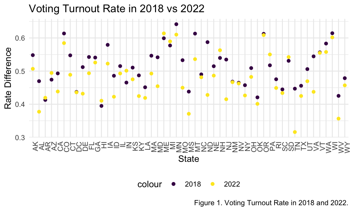
abortionvoting_df %>%
  drop_na() %>%
  ggplot(aes(x = state_abv)) +
    geom_point(aes(y = turnout_estimate2018, colour = "2018")) +
    geom_point(aes(y = turnout_estimate2022, colour = "2022")) +
  theme(axis.text.x = element_text(angle = 90, hjust = 1)) +
  labs(
    title = "Turnout Estimate Number in 2018 vs 2022",
    x = "State",
    y = "Rate Difference",
    caption = "Figure 2. Turnout Estimate Number in 2018 and 2022.")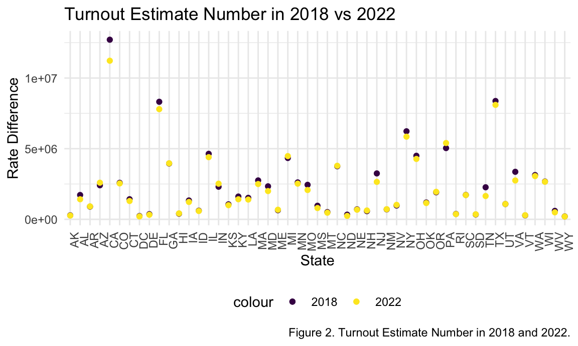
abortionvoting_df %>%
  drop_na() %>%
  ggplot(aes(x = state_abv)) +
    geom_point(aes(y = voting_eligible_pop2018, colour = "2018")) +
    geom_point(aes(y = voting_eligible_pop2022, colour = "2022")) +
  theme(axis.text.x = element_text(angle = 90, hjust = 1)) +
  labs(
    title = "Voting Eligibility Population in 2018 vs 2022",
    x = "State",
    y = "Population",
    caption = "Figure 3. Voting Eligibility Population in 2018 and 2022.")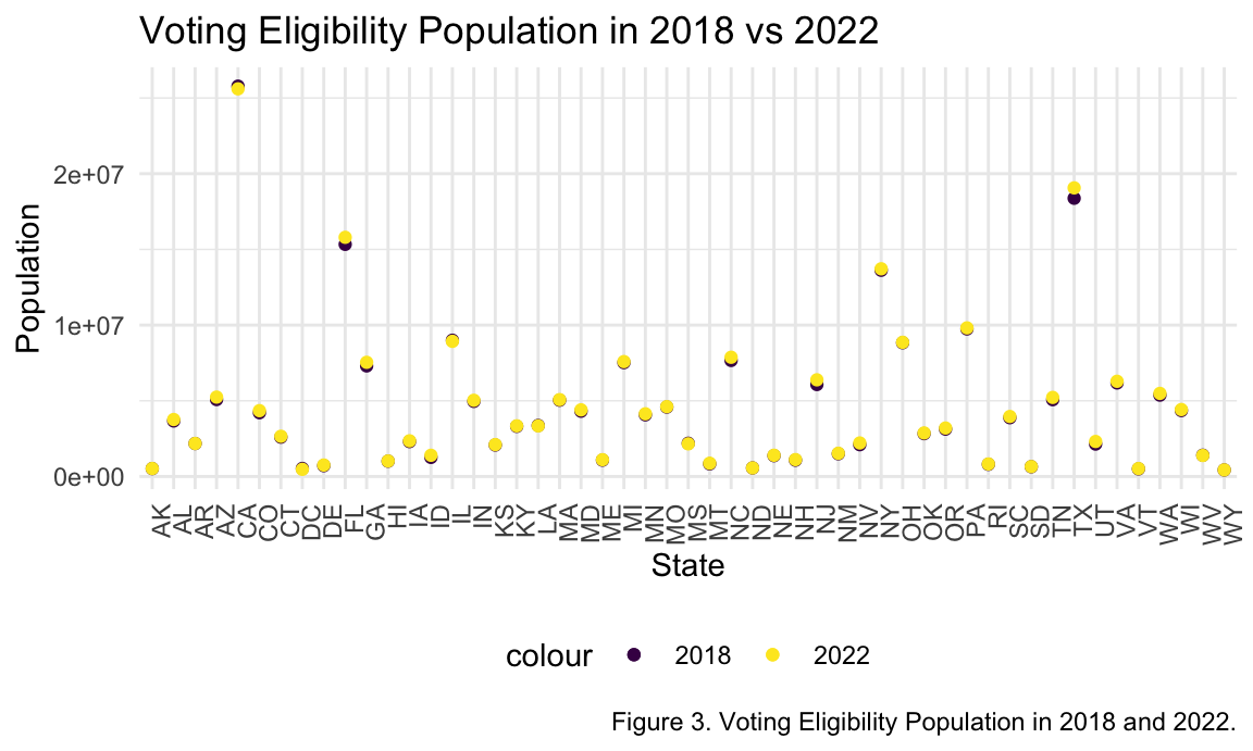
abortionvoting_df %>%
  drop_na() %>%
  ggplot(aes(x = state_abv)) +
    geom_point(aes(y = voting_age_pop2018, colour = "2018")) +
    geom_point(aes(y = voting_age_pop2022, colour = "2022")) +
  theme(axis.text.x = element_text(angle = 90, hjust = 1)) +
  labs(
    title = "Voting Age Population in 2018 vs 2022",
    x = "State",
    y = "Difference",
    caption = "Figure 4. Voting Age Population in 2018 and 2022.")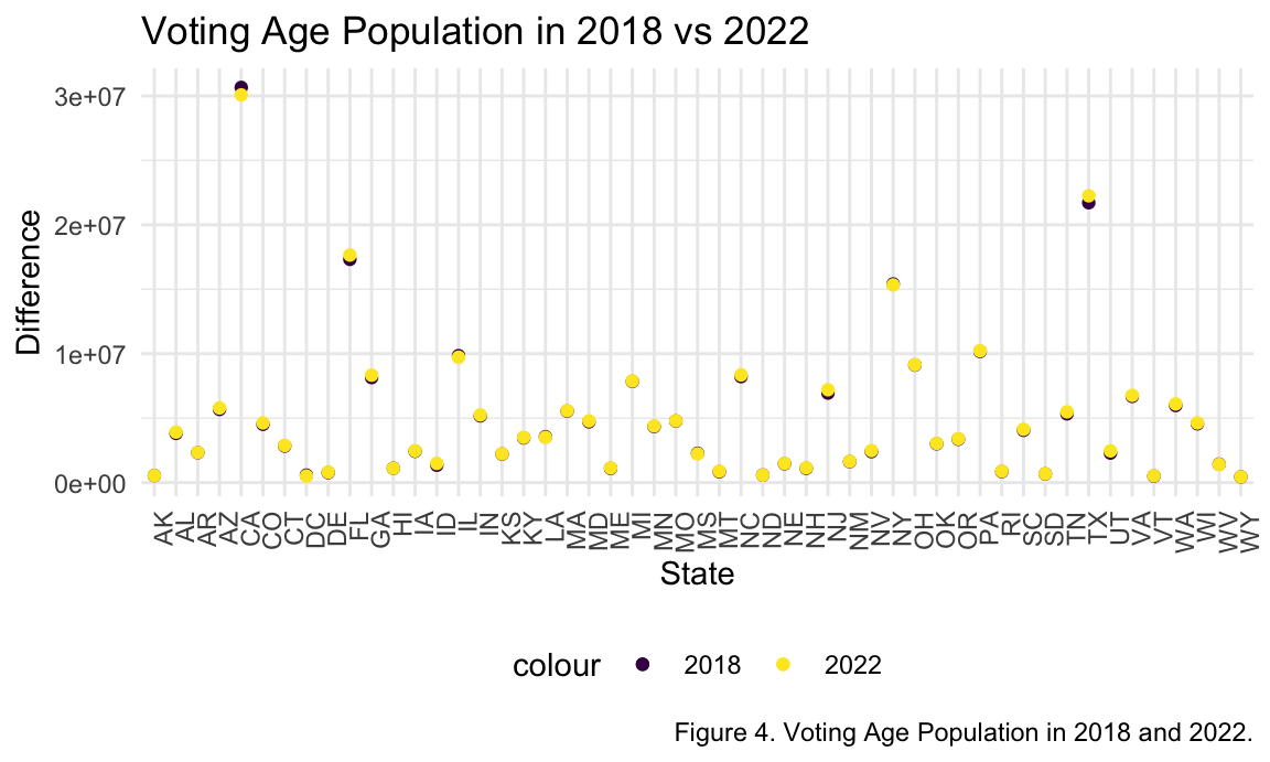
Abortion Laws and Accessibility Graphs
abortionvoting_df %>%
  drop_na() %>%
  ggplot(aes(x = state_abv)) +
  geom_point(aes(y = clinicdistance_jun, colour = "June")) +
  geom_point(aes(y = clinicdistance_jul, colour = "July")) +
  theme(axis.text.x = element_text(angle = 90, hjust = 1)) +
  labs(
    title = "Distance to an Abortion Provider from June to July, 2022",
    x = "State",
    y = "Distance (Miles)",
    caption = "Figure 5. Average Distance from an Abortion Clinic from June to July after Overturn of Roe vs. Wade.")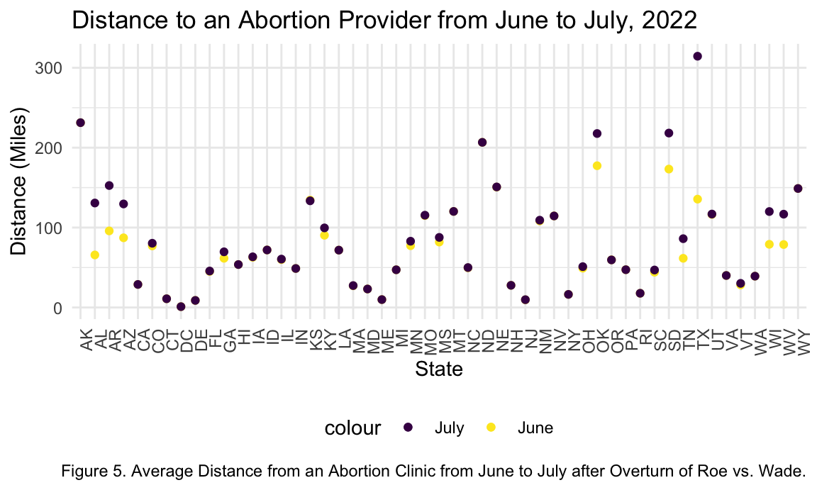
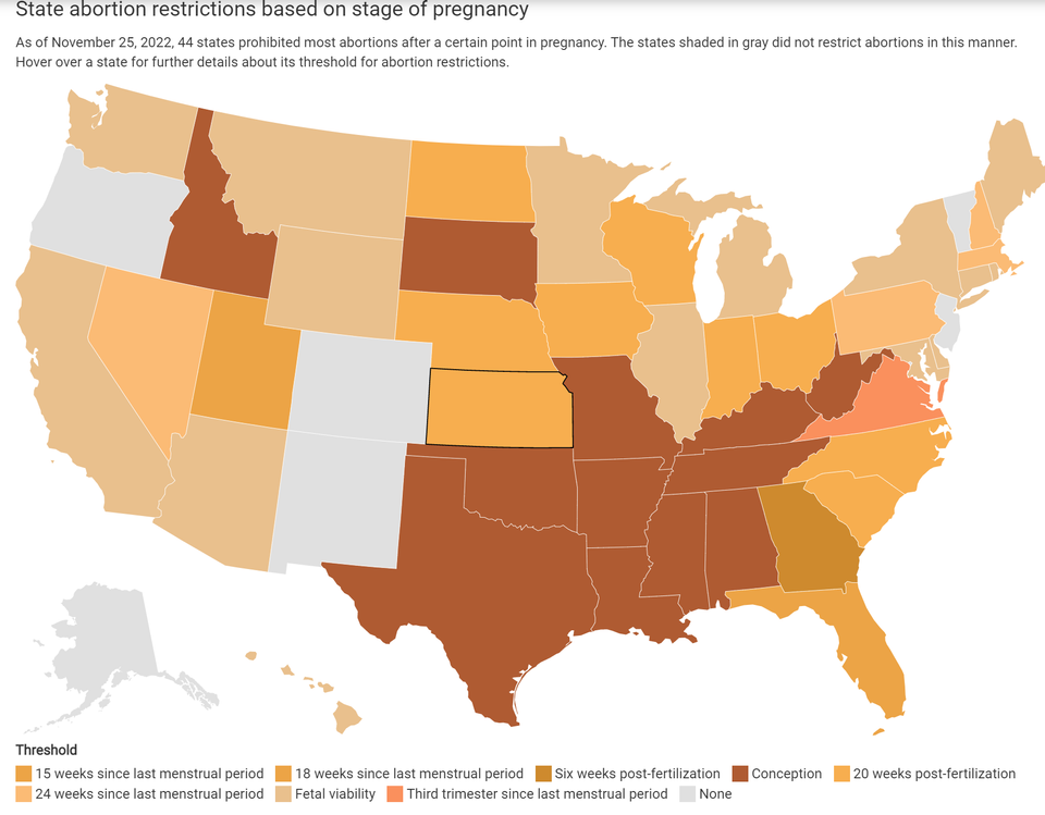
This figure from the Balletopedia dataset depicts state abortion restrictions based on the stage of pregnancy as of November 25, 2022. 44 states restricted abortions after a certain point in pregnancy, and 6 states including Washington D.C. did not implement any abortion restrictions. There are different thresholds on when abortion is restricted in the 44 states.
The definitions of the thresholds are explained below:
- Conception: prohibits all abortions, but abortion may be considered if the patient’s life is at risk.
- Fetal heartbeat: prohibits abortions after a fetal heartbeat can be detected; this may begin as soon as 6 weeks after the last menstrual period. Fetal viability: prohibits abortions and is interpreted by the Supreme Court at about 24-28 weeks into pregnancy.
- Last menstrual period: marks the beginning of a pregnancy from the first day of a woman’s last menstrual period (LMP).
- Post-fertilization: marks the beginning of conception, which can be up to 24 hours following intercourse.
- Post-implantation: marks the beginning of pregnancy and takes place when an egg attaches to the uterus; this is roughly five days after the egg is fertilized.
Source: Balletopedia.org
Regression Analysis
A variable, ab_change was created to quantify the change
in abortion restriction status per state (ab_change = 1 if
Roe v. Wade added an abortion restriction that was not previously in
place; ab_change = 0 if the overturning of Roe v. Wade did
not change abortion restrictions). This variable was created by taking
the difference between abortion restriction status in 2022 and 2018.
final_full =
  read_csv("data_cleaned/finalprojectfinaldataset.csv") %>%
  mutate(
    ab_change = abstatus22 - abstatus18
  )
A regression model was created utilizing the following:
- Outcome: The difference in percent turnout rate between 2018 and
2022 (
turnout_rate_difference) - Predictor: The difference in abortion restriction status by state
between 2018 and 2022 (
ab_change) - Predictor: The average difference in closest abortion clinic by
state between 2018 and 2022 (
dist_change)
regress_turnoutdif_full =
  lm(turnout_rate_difference ~ ab_change + dist_change, data = final_full)

summary(regress_turnoutdif_full)
confint(regress_turnoutdif_full)
Upon running the model, we find that the change in abortion status has a significant effect on voter turnout (P = 0.0261). On average, a state that had an abortion restriction put in place after the overturning of Roe v. Wade had a 5.661% greater voter turnout in the 2022 election compared to the 2018 election. We are 95% confident that the true increase in voter turnout falls between 0.703% and 10.619%.
The average change in distance to abortion clinic was not significant.
Discussion
The first set of questions we were interested in answering focused on abortion laws and accessibility. Unfortunately, as expected, we did see an increase in the average distance to a safe abortion provider in states such as Alabama, Arkansas and Oklahoma. These are states that have already had strict laws regarding abortion prior to the overturn of Roe v. Wade. With the overturn, accessibility to safe abortions has only become more inaccessible especially in Texas. In figure 5 we can see that the average distance to an Abortion Clinic dramatically increases from an average of ~140 miles to ~ 300 miles.
When assessing the voter turnout data, it was surprising to see that in most states, voter turnout was either the same in 2018 and 2022 or there was a lower voter turnout in 2022. This was interesting to note as the eligible population (figure 3) stayed the same in most states, with 2022 actually having a higher eligible population in 2022.
When looking at the relationship between abortion laws and abortion clinic accessibility and voter turnout, we see that change in abortion restrictions from 2018 to 2022 had a significant impact on voter turnout from the 2018 to 2022 election. Further research may find other datasets which take into account other confounding variables which may also have increased voter turnout. From these analyses we can come to a reasonable conclusion that the overturn of Roe v Wade had some influence on voter turnout in the midterm elections of 2022.
Limitations
The abortion laws datasets had a lot of missing data for the years 2019-2021 which limited our analysis to the years 2018 and 2022. This was not a major issue since we used voter turnout data on the same years for different reasons. Additionally, did not use the data on threshold for abortion restrictions (the week of gestation in which abortion is banned) in our models due to time restrictions and coding challenges. Some states had not fully finished counting their votes by the time the 2022 voting data was compiled so these are preliminary numbers though they were close to full count. Based on that we don’t expect a major change in our finding using the complete count data for the analysis.
Our models had other limitations. First, the predictor for abortion restrictions in 2022 only takes into account restrictions that had an immediate effect after the overturning of Roe v. Wade. The predictor did not take into account any state laws that were pending, up for referendum, or to be put into effect months after the overturning. Second, the models do not capture the nuances of abortion restrictions whether as a result of excluding the restriction threshold from the data or when abortion is allowed in cases of rape, incest, or harm to the mother’s life. Including these nuances would paint a more accurate picture of voter turnout based on each states’ exact situation. In connection to both these limitations, a more robust model could be created by utilizing a dataset with each states’ type of abortion restrictions, as well as whether a referendum for abortion access was included on a state’s ballot. Further predictors could be added, such as state political leaning in last presidential election, religious ideology, and other proxies for abortion access other than distance to clinic.